









Overview
When you collect data from a population at one point in time, you have a “snapshot.”
Cross-sectional studies capture that moment and allow you to ask: How prevalent is a specific condition or characteristic in the population, and is there an association between two variables measured at the same time?
This article demonstrates how to transform primary cross-sectional data into scientifically meaningful and interpretable research findings:
- How to summarise the data (descriptive analysis).
- How to find links (measures of association).
- How to detect traps (biases and confounders).
- How to interpret results without overstating what they tell us.
Descriptive Analysis: Painting the Picture
Before you look for relationships, you must first describe your “snapshot”. This is called descriptive analysis.
It answers the “Who, What, and Where” of your study sample.
- We use different summaries for different types of data:
- Categorical Data (Labels): Use proportions and percentages.
Example: In our sample of 100 patients, 30 (30%) had Type 2 Diabetes. 60 (60%) were female.
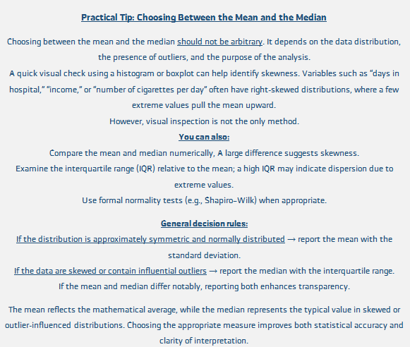
- Continuous Data (Numbers): Use means or medians.
- Mean: The “average” (add all values, then divide). Use it for data that is normally distributed (a “bell curve”).
Example: The mean age of the sample was 45.2 years.
- Median: The “middle value”, used when the data are not symmetrically distributed, typically due to the presence of extreme high or low values that distort the mean.”
Example: The median monthly income was $2,500. (Using the mean here might be misleading if one person earns $1,000,000).
- This is often “Table 1” in your research paper.
- It shows the basic characteristics of your sample (like age, gender, ethnicity, and other key variables). This table helps your reader understand exactly who you studied.
Measures of Association: Finding Links
- Now for the exciting part. Descriptive stats tell us what is. Measures of association tell us how things are related.
- In cross-sectional studies, we want to know if an exposure (e.g., smoking) is associated with an outcome (e.g., asthma).
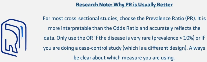
- The Prevalence Ratio (PR) is often the best and most intuitive measure for cross-sectional data analysis.
- Prevalence Ratio (PR): This directly compares the prevalence of the outcome in two groups.
- Formula:
- Example: Prevalence of asthma in smokers is 20%. Prevalence in non-smokers is 10%.
- Calculation: PR = 20% / 10% = 2.0.
- Interpretation: “Smokers are twice as likely to have asthma compared to non-smokers.” This is clear and easy to understand.
- Prevalence Difference (PD): This shows the absolute difference in prevalence.
- Calculation: PD = 20% – 10% = 10%.
- Interpretation: “There is a 10 percentage point excess of asthma prevalence among smokers.” This is very useful for public health planning.
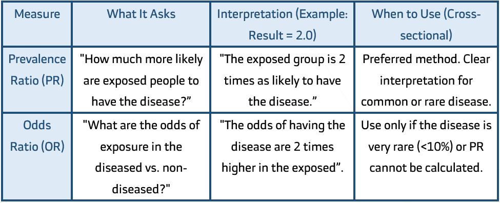
This table highlights the key differences when analyzing prevalence data
Recognizing Biases and Confounders
- Your data is rarely perfect. Biases and confounders are “hidden dangers” that can distort your results and lead to wrong conclusions.
- Sampling Bias (Selection Bias): Your study sample is not representative of the whole population.
Example: You study the prevalence of diabetes by surveying people at a specialty diabetes clinic. Your results will be far too high because you missed all the people without diabetes. - Response Bias (or Recall Bias): Participants answer questions inaccurately. This can be due to poor memory (recall) or social pressure (e.g., under-reporting alcohol use).
Example: People with a current health problem might think harder about past exposures than healthy people, creating a false link.
- A confounder is a “third variable” that is associated with both the exposure and the outcome, thereby distorting the true relationship between them.
- Illustrative Example: You find an association between high social media use (exposure) and poor sleep quality (outcome).
- The Confounder: Psychological stress.
- The Problem:
- Students experiencing high levels of stress may spend more time on social media and are also more likely to have poor sleep.
- If stress is not measured and adjusted for, the study may incorrectly attribute the sleep disturbance primarily to social media use, when stress is partially or largely responsible for the observed association.
For a variable to be considered a confounder, it must:
- Be associated with the exposure.
- Be independently associated with the outcome.
- Not lie on the causal pathway between exposure and outcome.
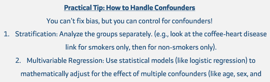
How to Control for Confounding:
- Confounding can be addressed at the design stage (restriction, matching) or during analysis using stratification or multivariable regression models. A practical rule is that if the adjusted estimate changes by ≥10% compared to the crude estimate, meaningful confounding is likely present.
Interpreting Results and Avoiding Over-interpretation
- This is the most critical step. How do you explain what you found without going too far?
Association Vs. Causation (The Golden Rule)
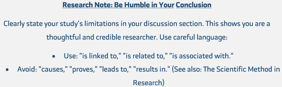
- The single biggest limitation of a cross-sectional study is that ASSOCIATION DOES NOT PROVE CAUSATION. Because you took a “snapshot,” you have a “chicken and egg” problem. You don’t know what came first.
- Scenario: You find a strong association between low physical activity and depression.
- Wrong Interpretation: “Low physical activity causes depression.”
- Correct Interpretation: “Low physical activity is associated with depression.”
- Alternative Explanations:
- Does inactivity lead to depression? (Possible)
- Does depression lead to inactivity? (Also possible)
- Does a third factor (like chronic pain) cause both depression and inactivity? (Confounding)
- A cross-sectional study cannot tell you which of these is true.
Considering Alternative Explanations
- Always be your own biggest critic. Before you claim a link, ask yourself:
- Could bias explain this finding?
- Could confounding explain this finding?
- Could this just be due to random chance?
Common Mistakes to Avoid
- Claiming Causation: The most common and serious error. You can only report an association because exposure and outcome are measured at the same time, so temporality cannot be established. Always use wording such as “associated with” instead of “caused by.”
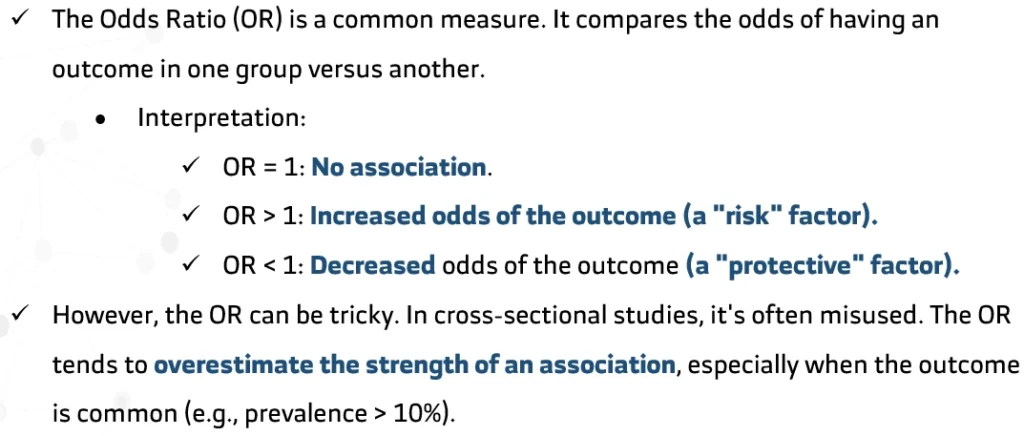
- Using Odds Ratio for a Common Outcome: This inflates your finding because Odds Ratios overestimate the association when outcome prevalence is high. As a rule, if prevalence is >10–20%, consider using the Prevalence Ratio (via log-binomial or Poisson regression with robust variance). Never interpret OR as “risk” when the outcome is common.
- Ignoring Confounders: Failing to adjust for known confounders (like age or sex) can bias your results. A practical rule: if the adjusted estimate changes by ≥10% compared to the crude estimate, confounding is likely present. Predefine confounders based on literature, not only statistical significance.
- Over-generalizing Results: If you studied 3rd-year medical students at one hospital, you cannot generalize your findings to all doctors in the country. External validity depends on sampling method and representativeness. Always clearly define your target population and limit conclusions accordingly.
Key Takeaways
- Cross-sectional studies are “snapshots” that measure prevalence and associations at one time.
- Start your analysis by describing your sample with means, medians, and proportions (Table 1).
- Use the Prevalence Ratio (PR) as your main measure of association. It’s more accurate and intuitive than the Odds Ratio.
- Always check for bias and control for confounding variables (like age, sex, or smoking).
- The golden rule: Association is NOT causation. Never forget the “chicken and egg” problem.
References
- Setia MS. Methodology Series Module 3: Cross-sectional Studies. Indian J Dermatol. 2016;61(3):261-264. doi:10.4103/0019-5154.182410 (PMID: 27293245)
- Lee J, Chia KS. Estimation of prevalence ratios in cross-sectional studies – an example from the 2016 Singapore National Health Survey. Ann Acad Med Singap. 2020;49(3):140-144. (PMID: 32296727)
- Canchola AJ, Stewart SL, Horn-Ross PL. Use of prevalence ratios and prevalence differences in the analysis of cross-sectional data. Am J Epidemiol. 2018;187(3):626-633. doi:10.1093/aje/kwx296 (PMID: 28911075)
- Wang X, Cheng Z. The impact of measurement error on the analysis of cross-sectional studies. Psychol Methods. 2020;25(6):703-720. doi:10.1037/met0000282 (PMID: 32191104)
- Tripepi G, Jager KJ, Dekker FW, Zoccali C. Confounding and effect modification: a primer for medical researchers. Nephrol Dial Transplant. 2021;36(11):2156-2162. doi:10.1093/ndt/gfaa172 (PMID: 32734283)
Authorship and Contributions
The following section acknowledges the individuals who contributed to the authorship, editing, translation, and preparation of this article, ensuring its academic integrity and clarity.
Dr. Ali Hmidoush
Author
M.D. and Medical Researcher; Director of Website & SEO Department at ResRef.
Dr. Ali Hmidoush
Author

Dr. Hani Harb
Editor
Professor of Infectious Immunology at TU Dresden, where he leads a dynamic research program at the interface of immunology, metabolism, and environmental health.
Dr. Hani Harb
Editor

Dr. Taha Al Khayrat
Translator & Formatter
A fifth-year medical student contributes to the Educational and Web departments at ResRef.
Dr. Taha Al Khayrat
Translator & Formatter